Equation of State
The momlevel package includes low-level NumPy functions as well as xarray-based wrappers to calculate in-situ density, derivatives of temperature and salinity with respect to density, and the thermal expansion / haline contraction coefficients. The implementation here uses the Wright (1997) equation of state (EOS), which is the default EOS used in MOM6 simulations. Other packages already exist to calculate these quantities, such as the Gibbs SeaWater (GSW) toolbox that uses the TEOS-10 EOS. While there is little fundamental difference between the two EOSs, attention must be paid to unit details such as conservative versus potential temperature and absolute versus practical salinity.
The Wright EOS implementation provided here is consistent with the EOS used in the model and is configured to use potential temperature referenced to the surface and practical salinity, which are directly output from the model.
Background
The Wright Equation of State (1997) is the default EOS used in MOM6 for climate applications. The EOS provides a formulation for in-situ density based on potential temperature, salinity, and pressure. This implementation is computationally efficient and targeted for use in numerical models.
The momlevel package is structured in modular way such that additional EOS implementations can be added to the momlevel.eos module. The low-level NumPy functions have a basic interface of (T, S, and p) and are optimized through the higher-level xarray functions in the package.
Calculating In situ Density
The example below illustrates how to calculate the in situ density (kg m-3) using potential temperature and salinity averaged over years 1980-1999 from the NOAA-GFDL CM4 historical CMIP6 simulation. Note that pressure is approximated as depth multiplied by 1e4.
In [1]: import xarray as xr

In [2]: xr.set_options(display_style="html")
Out[2]: <xarray.core.options.set_options at 0x7196aa0292b0>

In [3]: import momlevel

In [4]: import matplotlib.pyplot as plt

In [5]: import pkg_resources as pkgr

In [6]: example_dataset = pkgr.resource_filename(
   ...:     "momlevel",
   ...:     "resources/CM4_historical.nc"
   ...: )
   ...:

In [7]: ds = xr.open_dataset(example_dataset)

In [8]: ds
Out[8]:
<xarray.Dataset>
Dimensions:  (z_l: 35, lat: 180, lon: 360, z_i: 36)
Coordinates:
  * z_l      (z_l) float64 2.5 10.0 20.0 32.5 ... 5e+03 5.5e+03 6e+03 6.5e+03
  * lat      (lat) float64 -89.5 -88.5 -87.5 -86.5 -85.5 ... 86.5 87.5 88.5 89.5
  * lon      (lon) float64 0.5 1.5 2.5 3.5 4.5 ... 355.5 356.5 357.5 358.5 359.5
  * z_i      (z_i) float64 0.0 5.0 15.0 25.0 ... 5.75e+03 6.25e+03 6.75e+03
Data variables:
    thetao   (z_l, lat, lon) float32 ...
    so       (z_l, lat, lon) float32 ...
Density is calculated using the xarray front end momlevel.derived.calc_rho:
In [9]: rho = momlevel.derived.calc_rho(ds.thetao,ds.so,ds.z_l*1e4)

In [10]: rho.coords
Out[10]:
Coordinates:
  * z_l      (z_l) float64 2.5 10.0 20.0 32.5 ... 5e+03 5.5e+03 6e+03 6.5e+03
  * lat      (lat) float64 -89.5 -88.5 -87.5 -86.5 -85.5 ... 86.5 87.5 88.5 89.5
  * lon      (lon) float64 0.5 1.5 2.5 3.5 4.5 ... 355.5 356.5 357.5 358.5 359.5

In [11]: rho.attrs
Out[11]:
{'standard_name': 'sea_water_density',
 'long_name': 'In situ sea water density',
 'comment': 'calculated with the Wright equation of state',
 'units': 'kg m-3'}
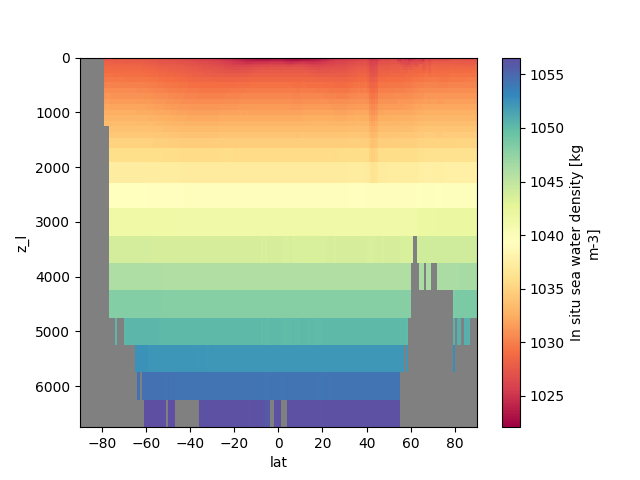
Here is a map of the zonal mean density:
In [12]: rho = rho.mean(dim="lon").assign_attrs(rho.attrs)

In [13]: fig = rho.plot(
   ....:     cmap="Spectral",
   ....:     yincrease=False,
   ....:     subplot_kws={"facecolor":"gray"}
   ....: )
   ....:
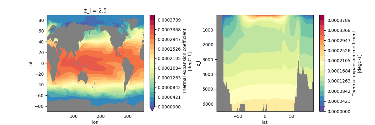
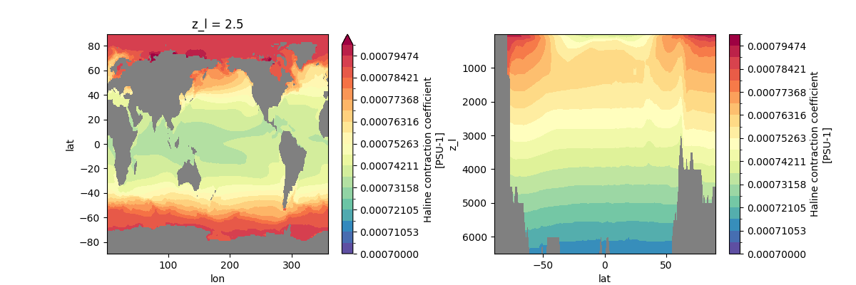
Thermal and Haline Expansion Coefficients
Thermal expansion coefficient (\(\alpha\)) and haline contraction coefficient (beta) are derived from the equation state. These quantities are typically involved in the calculation of buoyancy and stratification, i.e.:
but they are also relevant for sea level rise as discussed below. The naming convention follows that increasing temperature leads to a decrease in density (i.e. expansion) and that increasing salinity leads to an increase in density (i.e. contraction).
Definitions
The coefficients are calculated by taking the derivative of density with respect to either temperature or salinity while holding the other quantity fixed along with pressure.
Relationship to Sea Level
The coefficients can be interpreted as a “potential”, i.e. how much a given change in temperature or salinity can contribute locally to steric sea level change. In the absence of a transient scenario where heat or salt is added to the ocean, the rearrangement of existing water masses can contribute to non-zero density-driven sea level changes. This is one way in which changes in ocean circulation can impact sea level.
From Griffies et al. (2014), the coefficients are related to thermosteric and halosteric sea level change:
Where \(\eta\) is the sea level and \(-H\) is the sea floor
Note
These definitions of the local thermosteric and halosteric sea level change are different from the implementation used in the momlevel.steric module.
Calculating the Coefficients
In [14]: alpha = momlevel.derived.calc_alpha(ds.thetao,ds.so,ds.z_l*1e4)

In [15]: fig = plt.figure(figsize=(12,4))

In [16]: ax1 = plt.subplot(1,2,1, facecolor="gray")

In [17]: ax2 = plt.subplot(1,2,2, facecolor="gray")

In [18]: alpha_surf = alpha.isel(z_l=0)

In [19]: alpha_surf.plot.contourf(
   ....:     cmap="Spectral_r",
   ....:     vmin=0,
   ....:     vmax=0.0004,
   ....:     levels=20,
   ....:     ax=ax1
   ....: )
   ....:
Out[19]: <matplotlib.contour.QuadContourSet at 0x7196a88e85e0>

In [20]: alpha_xave = alpha.mean(dim="lon").assign_attrs(alpha.attrs)

In [21]: alpha_xave.plot.contourf(
   ....:     cmap="Spectral_r",
   ....:     vmin=0,
   ....:     vmax=0.0004,
   ....:     levels=20,
   ....:     yincrease=False,
   ....:     ax=ax2
   ....: )
   ....:
Out[21]: <matplotlib.contour.QuadContourSet at 0x7196a8cab760>

In [22]: plt.subplots_adjust(wspace=0.4)

In [23]: fig
Out[23]: <Figure size 1200x400 with 4 Axes>
In [24]: beta = momlevel.derived.calc_beta(ds.thetao,ds.so,ds.z_l*1e4)

In [25]: fig = plt.figure(figsize=(12,4))

In [26]: ax1 = plt.subplot(1,2,1, facecolor="gray")

In [27]: ax2 = plt.subplot(1,2,2, facecolor="gray")

In [28]: beta_surf = beta.isel(z_l=0)

In [29]: beta_surf.plot.contourf(
   ....:     cmap="Spectral_r",
   ....:     vmin=0.0007,
   ....:     vmax=0.0008,
   ....:     levels=20,
   ....:     ax=ax1
   ....: )
   ....:
Out[29]: <matplotlib.contour.QuadContourSet at 0x7196a3fc9eb0>

In [30]: beta_xave = beta.mean(dim="lon").assign_attrs(beta.attrs)

In [31]: beta_xave.plot.contourf(
   ....:     cmap="Spectral_r",
   ....:     vmin=0.0007,
   ....:     vmax=0.0008,
   ....:     levels=20,
   ....:     yincrease=False,
   ....:     ax=ax2
   ....: )
   ....:
Out[31]: <matplotlib.contour.QuadContourSet at 0x7196a398fd60>

In [32]: plt.subplots_adjust(wspace=0.4)

In [33]: fig
Out[33]: <Figure size 1200x400 with 4 Axes>
References
Griffies, S.M., et al., 2014: An assessment of global and regional sea level for years 1993–2007 in a suite of interannual CORE-II simulations. Ocean Modelling, 78, pp.35-89. https://doi.org/10.1016/j.ocemod.2014.03.004
Wright, D.G., 1997: An equation of state for use in ocean models: Eckart’s formula revisited. Journal of Atmospheric and Oceanic Technology, 14(3), pp.735-740. https://doi.org/10.1175/1520-0426(1997)014%3C0735:AEOSFU%3E2.0.CO;2