Tide Gauge Locations
The momlevel package includes functions for extracting ocean model output at specific tide gauge locations. The functionality takes into account the irregular grids common to ocean model output to find the best match between point locations and corresponding grid points. The momlevel package includes a default set of US-based tide gauge locations although users may specify their own locations.

Figure 1: United States tide gauge locations included in momlevel. Locations correspond to those considered in the projections provided by the Interagency Sea Level Rise Technical Report, Sweet et al. (2022).
Issues with Point Extraction
Ocean model output is typically presented on irregular grids such that the spacing between grid points in the x and y directions is not guaranteed to be uniform. These grids have 2-dimensional coordinate variables, e.g. geolat and geolon, that describe the true coordinates of the model grid points.
Warning
The geolon and geolat variables from MOM6 output represent the true coordinates of the grid cell. These variables should always be used when referencing the model output to real-world locations, such as for plotting and for point extraction.
The geolon and geolat variables are grid coordinates. This is notably different from the grid dimensions, e.g. xh and yh. Despite the latter having real-world resemblance, the grid dimensions can be more appropriately thought of as array indices.
Incorrect results can result when the xarray.core.DataArray.sel() method is used to extract grid points using the array-relative xh and yh dimensions.
Tide gauges are often located along coastlines at the interface between the land and ocean. Sometimes the nearest model grid point to a point location is not a valid ocean point. The tide gauge extraction in momlevel searches for the nearest valid ocean grid point.
Users can also specify a maximum distance between a real-world location and a model grid point. A threshold of 1.5 times the nominal model horizontal grid spacing is recommended for most applications. The distance between a point location and a model grid cell is calculated using a haversine, or great-circle, distance.
Example Usage
In this example, daily maximum sea surface height (ssh_max) is extracted for tide gauge locations in the Mid-Atlantic Bight. The sample model data for this example are spatial and temporal subset of a Regional MOM6 simulation run at 1/12-degree resolution
Loading Sample Data
import xarray as xr
import momlevel
import matplotlib.pyplot as plt
import pkg_resources as pkgr
%matplotlib inline

example_dataset = pkgr.resource_filename(
    "momlevel",
    "resources/NWA12_sample_grid_data.nc"
)
ds = xr.open_dataset(example_dataset)
ds
<xarray.Dataset>
Dimensions:       (yq: 146, xq: 101, yh: 146, xh: 100, time: 31, nv: 2)
Coordinates:
  * nv            (nv) float64 1.0 2.0
  * time          (time) datetime64[ns] 2008-01-01T12:00:00 ... 2008-01-31T12...
  * xh            (xh) float64 -76.96 -76.88 -76.8 ... -69.2 -69.12 -69.04
  * xq            (xq) float64 -77.0 -76.92 -76.84 ... -69.16 -69.08 -69.0
  * yh            (yh) float64 35.03 35.09 35.16 35.23 ... 43.84 43.9 43.96
  * yq            (yq) float64 35.06 35.13 35.19 35.26 ... 43.87 43.93 43.99
Data variables: (12/30)
    Coriolis      (yq, xq) float32 ...
    areacello     (yh, xh) float32 ...
    areacello_bu  (yq, xq) float32 ...
    areacello_cu  (yh, xq) float32 ...
    areacello_cv  (yq, xh) float32 ...
    average_DT    (time) timedelta64[ns] ...
    ...            ...
    ssh_max       (time, yh, xh) float32 ...
    time_bnds     (time, nv) timedelta64[ns] ...
    wet           (yh, xh) float32 ...
    wet_c         (yq, xq) float32 ...
    wet_u         (yh, xq) float32 ...
    wet_v         (yq, xh) float32 ...
Attributes:
    associated_files:  areacello: 20170101.ocean_static.nc
    grid_tile:         N/A
    grid_type:         regular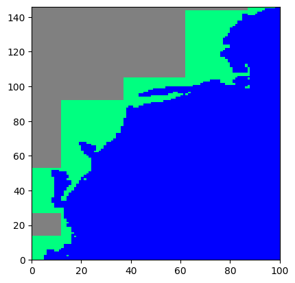
title: NWA12_euro_SADOURNY75_ENERGY_smag0.060_vel0.005_lap25_...The wet mask for this dataset illustrates a mixture of land, ocean, and undefined points:
fig = plt.figure()
ax = plt.subplot(1,1,1,aspect=0.7,facecolor="gray")
ax.pcolormesh(ds.wet,cmap="winter_r")
<matplotlib.collections.QuadMesh at 0x7f8087657790>
Extracting Data at Tide Gauge Locations
ds_tide_gauge = momlevel.extract_tidegauge(
    ds.ssh_max,
    ds.geolon,
    ds.geolat,
    mask=ds.wet,
    threshold=13.75
)

ds_tide_gauge
<xarray.Dataset>
Dimensions:              (time: 31)
Coordinates:
  * time                 (time) datetime64[ns] 2008-01-01T12:00:00 ... 2008-0...
Data variables: (12/16)
    ATLANTIC_CITY        (time) float32 -0.01668 -0.1694 ... 0.06807 -0.1113
    BRIDGEPORT           (time) float32 0.1712 -0.06221 ... 0.2597 0.02115
    CAPE_MAY             (time) float32 0.02824 -0.2248 ... 0.0521 -0.0655
    DUCK_PIER_OUTSIDE    (time) float32 -0.07135 -0.1315 ... -0.1331 -0.06825
    KIPTOPEKE_BEACH      (time) float32 -0.05812 -0.1867 ... -0.1044 -0.06178
    LEWES                (time) float32 -0.08047 -0.3301 ... -0.07797 -0.1678
    ...                   ...
    OREGON_INLET_MARINA  (time) float32 -0.0966 -0.1323 ... -0.1396 -0.07782
    PORTLAND             (time) float32 0.5883 0.5908 0.603 ... 0.7386 0.5683
    SANDY_HOOK           (time) float32 0.05917 -0.04586 ... 0.1779 -0.03983
    SEAVEY_ISLAND        (time) float32 0.5579 0.5733 0.5979 ... 0.6966 0.5575
    SEWELLS_POINT        (time) float32 -0.1529 -0.2656 ... -0.2527 -0.07424
SOLOMONS_ISLAND (time) float32 -0.1853 -0.3871 ... -0.116 -0.3836Each array in the output dataset includes additional attributes that describe the results of the translation of point locations to the model grid:
name: Site name, also the same as Permanent Service for Mean Sea Level (PSMSL) station nameNOAA_name: NOAA tide gauge station namePSMSLID: Permanent Service for Mean Sea Level station id numberNOAAID: NOAA tide gauge station id numberdistance: distance between tide gauge location and grid cell center, in kmmod_index: integer index of the model’s flattened x-y grid arraymodel_coords: lat-lon coordinates from the model grid (i.e.geolat,geolon)dims: y-x dimension namesdim_vals: y-x dimension values from the model grid (i.e.yh,xh)real_coords: real coordinates of tide gauge location
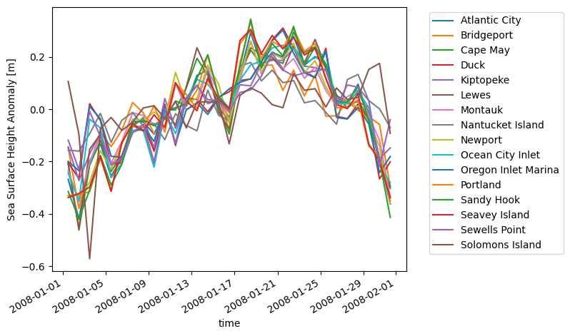
Plotting Location Timeseries
fig = plt.figure()
ax = plt.subplot(1,1,1)
for var in ds_tide_gauge.keys():
    var = ds_tide_gauge[var]
    (var - var.mean()).plot(ax=ax,label=var.NOAA_name)
plt.legend()
ax.set_ylabel("Sea Surface Height Anomaly [m]")
ax.legend(bbox_to_anchor=(1.05, 1))
<matplotlib.legend.Legend at 0x7f80843881f0>
References
Sweet, W.V., B.D. Hamlington, R.E. Kopp, C.P. Weaver, P.L. Barnard, D. Bekaert, W. Brooks, M. Craghan, G. Dusek, T. Frederikse, G. Garner, A.S. Genz, J.P. Krasting, E. Larour, D. Marcy, J.J. Marra, J. Obeysekera, M. Osler, M. Pendleton, D. Roman, L. Schmied, W. Veatch, K.D. White, and C. Zuzak, 2022: Global and Regional Sea Level Rise Scenarios for the United States: Updated Mean Projections and Extreme Water Level Probabilities Along U.S. Coastlines. NOAA Technical Report NOS 01. National Oceanic and Atmospheric Administration, National Ocean Service, Silver Spring, MD, 111 pp. https://oceanservice.noaa.gov/hazards/sealevelrise/noaa-nos-techrpt01-global-regional-SLR-scenarios-US.pdf